
Even though the current probe pre-compliance test method I’m about to describe has been documented and presented for decades, in my experience it’s an incredible tool that is still rarely used by manufacturers.
This affordable and simple technique should really be undertaken on EVERY. SINGLE. PRODUCT. BEFORE you send it to an EMC test lab. It’s quick, it’s easy, and it has great correlation to fully compliant radiated emissions measurements.
It can tell you if your product is likely to pass or fail with a high degree of accuracy. So why would you not use this?
Let’s find out what it’s all about!
In this article we’re going to learn:
- What are current probes?
- What is common-mode current?
- How accurate is the e-field extrapolation from a current probe?
- Required test equipment
- How to make the measurements
- How to extrapolate to electric field strength
- A spreadsheet tool to quickly determine pass/fail
What are current probes?
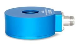
TekBox Current Probe
Current probes are essentially RF current transformers. If you imagine a standard transformer with isolated primary and secondary windings, the current probe is equivalent to one of the winding sides.
When a probe is clamped around a cable, the conductor can be considered the primary winding (a single turn) and the probe’s windings are the secondary. It is the magnetic flux generated by the varying RF current in the cable that are picked up by the current probe through the mutual coupling inductance.
Current measurements are made by having the current carrying conductor pass through the aperture of the probe and the probe’s output voltage is measured using a spectrum analyzer (or field intensity meter).
The transfer impedance data (provided with any characterized probe) can then be used to convert the reading from the analyzer to a current as follows:
dBμA = dBμV – Transfer Impedance (dBΩ)
You could make your own probe using a toroidal ferrite, some wire and a BNC connector, but now that low cost suppliers such as TekBox offer these probes at <50% of traditional pricing, it becomes harder to justify the time making and characterizing a probe yourself.
We’ll cover how to convert this to a far-field electric field strength measurement shortly.
Why Current Probe Measurements?
An age-old value proposition made by EMC test equipment manufacturers about why you should buy their product is that if they can save you even one day in a test lab, it’s worth the cost of their product.
The main objection to this is usually whether that is actually true. Maybe it is, maybe it isn’t. The claim is hard to quantify.
In the case of a properly characterized current probe used in conjunction with a basic spectrum analyzer, that value proposition is about as true as it ever gets. With a total cost in the region of 0.5 to 1 day worth of test lab time and with very repeatable and accurate extrapolated results (data from a paper below), the ROI can be justified on just one product development cycle. Amortized over several products, it becomes even more of a no-brainer.
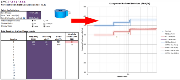
As shown in the figure below, it’s possible to use the frequency, cable length, probe transfer impedance and spectrum analyzer reading to extrapolate to a far-field radiated electric field strength reading that can be compared directly with standard limits (FCC and CISPR22 Class A/B shown).
Using Current Probe Measurements to Extrapolate to Radiated E-Field Strength
So what makes these probes so useful?
What led Henry Ott to say “Of all the various types of EMC measurements that you could possibly do, the common-mode current measurement is the most useful.”?
In this article, I’ll be discussing the current probe in relation to radiated emissions pre-compliance testing. They can also be used for troubleshooting, but that isn’t the purpose of this article.
For a pre-compliance tool to be useful, ideally it needs to correlate very well with final compliance measurements. Current probes are one of the few tools we have that can be used to accurately predict final measurements.
The reason for that is that the predominant failure mode for unintentional radiated emissions testing (up to a few hundred MHz) is common-mode currents on external cabling.
Common-Mode Current Cable Radiation
Mighty tomes such as “Electromagnetic Compatibility Engineering” by Henry Ott often quote a guideline of approximately 5-15uA of measured current equating to a radiated emissions failure. But that very much depends on the frequency of the emission, the limits of the test standard you’re using and the length of the cable. We’ll look at those variables later in this article.
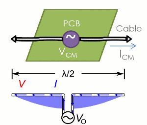
Cables are very good radiators because they’re typically the longest conductive structure in a given device and that makes them relatively more efficient at radiating radio waves.
If we want to intentionally radiate energy we use antennas and a very standard antenna configuration is a half-wave dipole. The maximum radiation efficiency happens (along with other criteria) when the dipole elements are exactly 1/2 of a wavelength because that allows the maximum voltage differential from tip to tip.
Our external cables can begin to look a lot like antennas with the driving source being circuitry that sits in the centre. Perhaps the driving source is a noisy ground plane that connects to cable shields on two cables.
What is common-mode current you ask?
Common-mode current as it relates to hardware design can be thought of as the unwanted current that flows ‘through’ parasitic capacitances that exist between the product and conductive structures in the outside world.
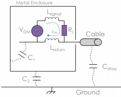
DM to CM Conversion (Current Driven Source Model)
To avoid breaking Kirchoff’s current law, a current loop still exists, just the current loop includes external structures (e.g. a building conduit, ground planes, metal cabinets etc..) and parasitic capacitances.
As the figure to the left illustrates, one way of modelling common-mode currents is to take an intentionally driven differential mode voltage source (e.g. a CMOS gate driver) and converting it to an equivalent common-mode current. This model is known as a current driven source model and an approximation of the common-mode current can be calculated using the equation below:
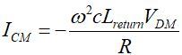
CM Current Approximation
One of the most common-ways of increasing the factor ‘Lreturn’ on a circuit board is to run a digital switching signal over a cut in a reference plane on the adjacent layer. The increased path length and loop area of the return current by definition increases the partial inductance in the return path.
How accurately can I extrapolate measurements to an electric field strength?
First thing to keep in mind is that variation in radiated emissions measurements can be quite large even between two accredited EMC test facilities. The maximum NSA (normalized site attenuation survey) deviation mandated by the FCC for example is +/- 4dB (so results may differ by 8 dB between test sites). In reality it may be higher than this.
If a method can get within +/- 4dB of measurements made at an accredited test site then that method is as good as another accredited test site.
3 Different Extrapolation Methods
The paper “Radiation from Common Mode Currents – Beyond 1 GHz” by M. Aschenberg and C. Grasso explores 3 extrapolation methods and compares their correlation to radiated emission measurements.
Method #1: Standard Approach
This is the method outlined by H. Ott and C. Paul in their textbooks. It’s a derivation/simplification of the full treatment outlined in “Antenna Theory – Analysis and Design” (C. Balanis).
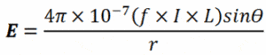
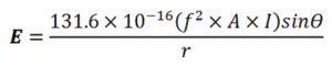
Electric Field Strength Calculation (*)
Although it’s very simple to use and apply, a limitation of this approach is that it assumes that the cables involved are electrically small, which is to say that their length is not a significant fraction of a wavelength.
As the frequency of the emission increases, the wavelength becomes smaller and the cables become a more significant fraction of that wavelength. This makes correlation above 100MHz – 200MHz increasingly inaccurate.
It is not true to say that emissions will get worse continuously as the cable length increases to infinity. In reality the emissions due to common-mode current on cabling ‘peak’ as the cable length approaches 1/2 wavelength of the noise frequency.
(*)
f = Frequency (Hz)
I = CM current (A)
L = Cable length (m)
r = Measurement distance (m)
θ = π/2
This method is very accurate up until approximately 200 MHz with a 1m cable.
Method #2: Balanis – Thin Wire Dipole
A more accurate method that doesn’t include approximations such as those used in method #1 above is described by Constantine Balais in “Antenna Theory – Analysis and Design”.
Unfortunately this method introduces complexities such as the effect of the ground plane and cable angle which make it impractical to use in real life.
This method is accurate beyond 1 GHz but comes with the downside of fairly un-achievable complexity.
Method #3: The Plateau
A hybrid of method #1 and #2 is described in “Radiation from Common Mode Currents – Beyond 1 GHz” by M. Aschenberg and C. Grasso which basically truncates the conversion factor at the maximum cable length of λ/2. At this point any increase in cable length does not increase the calculated E-field strength.
Watch as I increase the cable length below and see how the electric field strength of measurements increases up until the cable length exceeds λ/2. Notice how only the lower frequency emission increases when the cable length increases from 1m -> 2m, then neither emission increases from 2m -> 3m.
 This simple modification to method #1 vastly improves the correlation above 200 MHz and brings it within a few dB of the much more complex Balanis method.
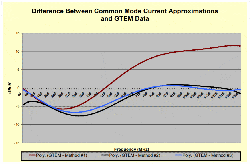
Comparison of the 3 Methods
Using a noise source and GTEM measurements for comparison, we can see that method #3 gives excellent correlation to GTEM radiated measurements.
For the most part, the deviation between method #3 and the GTEM measurements are within +2dB/-7dB! Not too bad when you recall that an accredited lab NSA deviation is +/- 4dB.
It’s worth noting that GTEM measurements have their own correlation to an OATS or chamber measurements. The graph below is taken from “The Use of GTEM Cells for EMC Measurements” by National Physical Laboratory and York EMC Services Ltd.
If used correctly, a GTEM can provide a really good correlation to an OATS or chamber so the comparison above can be taken as valid.
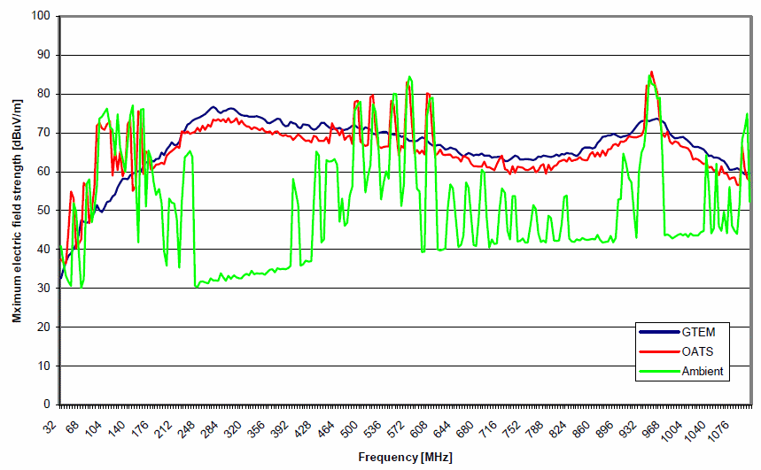
GTEM to 10m OATS comparison using CNEIII noise source (Source)
Usefulness as Frequency Increases
As noise frequencies increase, their wavelengths decrease. At 1 GHz for example λ/2 = 15 cm. At these wavelengths, enclosures and conductive structures on circuit boards themselves can become very efficient antennas. So we can say that as frequencies increase, common-mode current on external cabling becomes a smaller proportion of overall failure modes.
E-Field Extrapolation From a Differential Mode Current Source
Another reason that the current probe pre-compliance method becomes less useful as frequency increases is that wanted differential mode current sources begin to act as more efficient antennas in the region of a few hundred MHz and up. The reason being that there is an ‘f-squared’ term in the extrapolation equation shown to the left. The ‘f-squared’ term trumps the common-mode extrapolation’s linear ‘f’ term when the frequency reaches approximately 500-700 MHz depending on the loop area and currents involved.
That is not to say that if you measure common-mode current on a cable at 1 GHz and the extrapolated electric field strength is greater than the limit, you won’t fail radiated emissions testing. You probably will. It just means that you will catch a lower percentage of the failures above a few hundred MHz because more of those failures are not related to common-mode currents on external cabling.
Ultimately, the upper frequency boundary of the current probe method will likely be dictated by the transfer impedance of the probe you select. Most probes are sensitive up to a few hundred MHz, although some extend to 1 GHz and beyond. But if the sensitivity is too low then at some point the measurements will drop below the noise floor of your analyzer.
As a general guideline, I would recommend using a current probe to measure common-mode currents between 30 MHz and ~500 MHz.
How to make accurate measurements with a current probe
Here’s a summary of the test procedure and calculations:
- Clamp your chosen probe over a cable.
- Use bubble wrap or other non-conductive material to centre cable in probe hole.
- Move probe back and forth along cable to find maximum reading.
- Take reading off analyzer screen in dBuV.
- Calculate dBμA using: dBμA = dBμV – Transfer Impedance (dBΩ).
- Convert dBμA to A using: 10ˆ((dBμA-120)/20). This gives you I(cm).
- Plug I(cm) into this equation (method #1 above) to get E-Field in V/m:
- Convert V/m to dBuV/m using: 20*log(I(cm))+120.
- Compare to the field strength limit at the noise frequency in your standard. E.g. those defined in FCC 15.109.
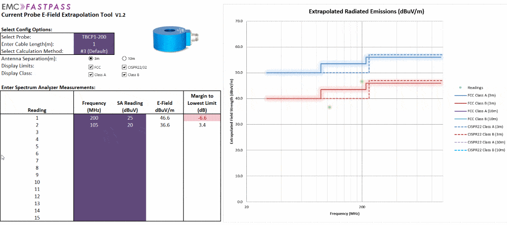
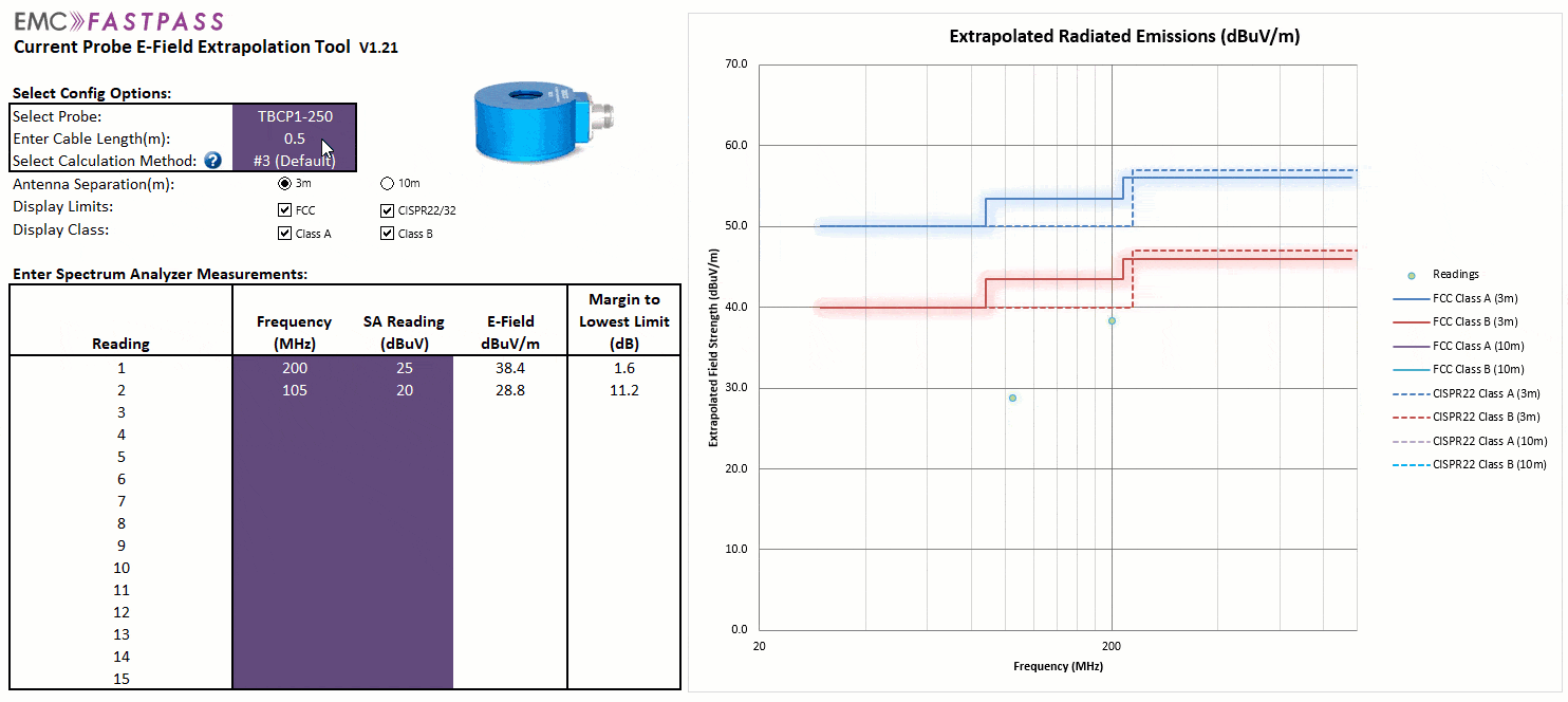
The calculations are quite easy to do if you set up a spreadsheet, but I found that taking into account the probe transfer impedance and emissions limit at each specific noise frequency took time and led to some mistakes. That’s why I developed a more sophisticated spreadsheet tool that allows you to enter probe characteristics over the frequency range as well as selecting the extrapolation method and relevant measurement distance and limits. It’s available for sale here along with the TekBox current probes here.
Summary
If you don’t already integrate current probe measurements into your standard pre-compliance testing process, hopefully this article shed some light on how useful and easy it can be.
Have you used one before? How useful did you find it? Let me know in the comments below.
Comments 20
Hi Andy
Wonderful compilation of core technical stuffs were put at one place, I appreciate your efforts and hardwork.
Thanks for educating us with the core of electromagnetics.
Regards,
Manish Kothari
From India
Author
You’re welcome Manish!
Hi Andy,
We are having a debate here where I work. We have been using the current probe method to test our devices before heading up to UL for formal testing. However, we have recently acquired a three meter EMC chamber.
Would it be better to still use the current probe or the EMC chamber? It seems to me that at a minimum using the EMC chamber would be significantly faster.
thanks for your article,
Josh
Author
Hi Josh,
If your 3m is fully compliant, or even a good pre-compliance chamber (with ~ +/- 6dB NSA deviation) then I would probably skip the current probe method to save time as you say. You could always use a comb generator to build confidence in the correlation between the current probe method, your chamber, and the final compliance chamber measurements in the same way as Aschenberg in the paper mentioned in the article.
https://www.emcfastpass.com/test-equipment/shop/comb-generators/comb-generator-frequency-multiplier-tbcg2/
Hi Andy,
thanks for posting very informative article on Current probes. Can i have pdf of the article.
Kanwal Jawanda
Formerly – Director R&D EMSCAN
Andy, thanks for posting this. Understanding the utility of the current probe for EMC pre-compliance testing is vital knowledge for all product designers!
Author
Thanks Ken. Your great articles on the subject served as some inspiration!
Hi Andy, thanks for sharing your methodology with us!
Do you have any reading suggestion to use a similar approach to correlate the near-field probe antenna measurements with the far-field radiated electric field strength?
Author
There is no way to do that. You would need the E-field, H-field and phase difference to be able to extrapolate from the near field measurements only. This is because the near-field does not always become a propagating wave.
Pingback: TEM Cell and GTEM Guide For Radiated Emissions & Radiated Immunity Pre-Compliance Testing - EMC FastPass
Pingback: TEM Cell and GTEM Guide For Radiated Emissions and Radiated Immunity Pre-Compliance Testing – iNARTE
Pingback: Minimizing EMI from LED Lighting – Case Study | EMC FastPass
Hi Andy,
thank you for your very useful and clear articles on EMC topics;
in your article on EMC chambers (‘Importance of absorber placement’)
you say that it is possible to partially line the chamber with ferrite tiles;
do you have some suggestion (or some reference text) to define
the best positioning?
Thank you in advance for your reply, best regards
Franco
Hi Andy
thank you for share, it is great.
one question about “Move probe back and forth along cable to find maximum reading”
it seams like different frequency has different level with different probe position along the cable.
can you help to explain the reason about this.
thank you
BR
Hi Andy,
Thanks for providing useful information for EMC testing.
I want to measure E-field response of current emission probe (10kHz to 400MHz).
Can you please share test procedure how can I do this?
Thank you
Pingback: 12 Ways to Expose Hidden Signals - EMC FastPass
Hi Andy,
Could the measurement method be used with much longer cable?
On my example it would be evaluating radiated noise on a 100m cable transporting dc voltage (twisted pair). Lab results in chamber show emission from 30 up to 200MHz.
For the radiated and conducted testing the cable is coiled in a least inductive mode (coiled in 8 shape approximately 80 cm long).
With this length, would the method of truncating the conversion factor at λ/2 = 1.5MHz would work? Is there any workaround possible with the coiled cable or do i have to go with the #2 method?
Thank you in advance,
Best regards,
Cyril
Small nitpick here, but step #6 has an error:
“Convert dBμA to A using: 10ˆ(dBμA-120)/20. This gives you I(cm).”
Per order of operations the above equation is incorrect. You want to add some paratheses:
10ˆ((dBμA-120)/20)
I was writing a python script to do all this stuff and I was way off on my Amperes calculation.
Great article, thank you!
Pingback: Self-Build EMC and Microwave Chambers - EMC FastPass
Hi Andy,
Thank you for the detailed introduction about current measurement.
And here I got a quesiton about the current measruement step 3:
“Move probe back and forth along cable to find maximum reading.”
Could you please share why to move probe back and forth? and what purpose to find maximum reading here?
Thanks in advance.
Donny