
Often it’s the case where it’s tough to find a noise source above the noise floor of your receiver or spectrum analyzer. Perhaps you have a test report from an EMC test lab and you’d like to troubleshoot the issue back at your office but you can’t find the emission using the equipment you have on-hand.
In this article I’ll dive into several simple ways to increase measurement sensitivity and lower your noise floor, effectively allowing you to ‘see’ much smaller signals.
I also made a short video that explores 3 of the methods described in this article, and you can view the video below.
Example of High vs Low Noise Floor
The plots below are taken from the same product, measured at 2 different EMC labs.
The first plot basically shows the noise floor and ambient level of the chamber and measurement setup. Emissions from the EUT are negligible.
Plot Showing Noise Floor of Anechoic Chamber
Very Low Noise Floor Measurement Exposes A Very Low Level Emission
With a combination of the items we’ll cover below, the second test lab shows a noise floor that is approximately 20 dB – 25 dB lower than the first, exposing much weaker emissions from the product.
Notice that the emissions (shown in light green in the second plot) has a level of around 18 dBuV/m at 200 MHz. This is not visible in the first plot because the noise floor is above this level.
Use a More Sensitive Transducer
Probably the most obvious place to start is to use a more sensitive transducer.
Antennas
In the case of an antenna, this means to use a higher gain antenna.
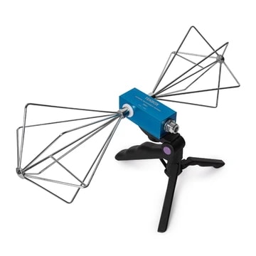
Biconical Antenna For EMI Testing
‘Gain’, in relation to a passive antenna does not mean higher amplification which the word may imply. Instead, it means higher ‘directionality’, and so a high gain passive antenna is more directional than a lower gain passive antenna.
If you’re using a hybrid biconical/log-periodic antenna, but you’re focusing on an emission that is under 300 MHz, then using a biconical antenna may offer higher gain by several dB.
Current Probe Transfer Function
In the case of a current monitor probe, which can be used to very effectively extrapolate to far-field electric field strength measurements, you may want to try a probe with a higher transfer impedance. A probe with a higher transfer impedance is more sensitive and will convert a given RF current into a higher voltage for the spectrum analyzer to measure.
Comparison of Transfer Impedance of 3 Different RF Current Monitor Probes
A higher transfer impedance equates to a higher sensitivity probe. So as you can see from the plots above, the TBCP1-500 is more sensitive than the -250 or -200 probes.
See the ‘Current probe pre-compliance testing guide‘ for more details on this method.
Near-Field Probe Size
In the case of a near-field inductive probe, by using a larger loop area you will inductively couple more of the noise signal. This comes at the cost of reducing the positional resolution of the probe (i.e. it’s harder to distinguish exactly where the emission is originating), but it may allow you to find an otherwise invisible emission.
Orientation and position of the probe can also make a huge different to the amount of signal pickup. In the case of magnetic field probes, the maximum coupling between the field source and the probe occurs when the overlapping loop area is maximized. This maximizes the mutual inductance and allows for maximum coupling. If you’re not picking up what you expect, try rotating the probe 90 degrees and/or re-orienting your probe horizontally instead of vertically.
Change the Antenna Polarization
In a similar way, if you’re using an antenna to make radiated emissions measurements, try orienting your antenna vertically instead of horizontally.
If the signal you’re trying to measure is below a few hundred MHz, very often it is the result of common-mode RF currents flowing on cabling attached to your product. Radiated emissions test setups usually require you to position the cabling to drape over the back of your test table which means that the antenna element (the cable) is oriented vertically, which in turn produces a vertically polarized electric field in the far-field region.
By orienting the ‘receive’ antenna in the same polarization, the RF voltage differential from tip-to-tip of your antenna will maximize the pickup of the transmitted signal.
Match Antenna to Cable Polarization to Maximize Signal Pickup
The difference in amplitude of the measured signal can easily vary by 10-20dB between horizontal and vertical antenna polarizations, which can make the difference between an emission being above or below the noise floor.
Choose Cabling Wisely
The type and length of coax cable you use can have an impact on your measured signal. Many different types are available and their RF performance varies significantly.
As you begin to work with higher frequencies, the cable choice becomes much more important. Signal attenuation per unit length is the important characteristic. For measurements under a few hundred MHz, standard coax type RG-58 will be fine, but as you extend into the multi-gigahertz region and beyond, attenuation can become significant.
Cable Type Attenuation Comparison [Source: AH Systems]
Use High Quality Adaptors
If you’re using adaptors to transition from connector to connector types (e.g. N-type to SMA), you can expect a small loss at the connector.
RF Adaptor Set
Below a few hundred MHz, you could measure a 0.5 to 1dB signal attenuation. But as you increase the frequency, the loss can become more significant.
You’ll find cheap RF adaptors as well as more expensive ones. I’ve observed differences of a couple of dB between adaptors, so if you want to achieve the most sensitive measurement setup, investing in high quality adaptors is important.
Another important factor is the type of connector you select. For many EMC/EMI applications, the N-type connector is used. It has good power handling capability (useful for radiated and conducted susceptibility), but the geometry of the connector limits the upper frequency range.
Upper Frequency Limit of Connector Types
As you can see from this chart, the frequency range of different connector types varies significantly, making a difference to attenuation especially as the frequency increases past a GHz or so.
Standardize Impedances to Avoid Mismatches
One ‘gotcha’ that can affect the amplitude and quality of signal transported to your analyzer is to accidentally use impedance mismatched cables or connectors.
The typical input impedance of a spectrum analyzer or receiver is 50 Ohms, although 75 Ohm analyzers do exist. For maximum power transfer in a system, the impedances must remain constant. So in a 50 Ohm system, that necessitates using coax and connectors with 50 Ohm characteristic impedance.
If you accidentally use a 75 Ohm component (cable, connector, attenuator, transducer etc.) in your 50 Ohm system, you’ll have an impedance mismatch which will degrade the signal reaching your analyzer.
Move Antenna Closer
For radiated measurements, a very simple method of increasing the measured signal is to physically move the antenna close to the EUT (equipment under test).
Test standards often allow for compliant measurements taken at 3m and 10m separations (between the EUT and the measurement antenna). The standards typically assume an inverse distance fall-off (1/r) of 20dB per decade. However, there have been many investigations into the validity of this and the fall-off has been shown to vary massively depending on EUT size, frequency range and polarization. This article by Daniel Hollihan goes into detail on this relationship.
As you move the measurement antenna into the near-field zone, the coupling mechanism will transition from an elecro-magnetic plane wave to predominantly capacitive or inductive, and measurements will become less repeatable. This is the reason that accredited test facilities use a minimum measurement separation of 3 metres (ideally 10m or 30m) for most radiated tests (except perhaps low frequency tests with monopoles or loop antennas).
For troubleshooting or pre-compliance purposes, measurements at 1 metre should be repeatable enough to measure the difference before and after mitigation techniques have been applied.
Use a Current Monitor Probe Instead of an Antenna
Sometimes using an antenna for measurements in your office is not practical. Perhaps there are significant ambient signals floating around such as Wi-Fi, cell phone and FM signals which drown out the signal you’re trying to measure.
As I mentioned earlier, for signals below a few hundred MHz, the predominant cause of radiated emissions failures is common-mode currents on external cabling. So instead of using an antenna, you can often use a cable current monitor probe instead.
These are less susceptible to ambient noise and can enable measurement of extremely small cable currents in the order of uA or nA.
Extrapolating Current Probe Measurements to Far-Field Measurements
As you can see above, cable current measurements can be used to extrapolate to far-field measurements and allow for comparison to regulatory limits.
See the ‘Current probe pre-compliance testing guide‘ for more details on this method.
Use a Pre-Amplifier
Another tool we can use to measure smaller signals is a microwave amplifier.
20dB RF Pre-Amplifier
These cost effective amps can boost our received signal by a significant amount (typically 20-40 dB).
By placing the pre-amp at the transducer (antenna) end of the cable, this will maximize the signal to noise ratio.
Often spectrum analyzers include an internal pre-amplifier option, in which case you can use this to increase sensitivity and lower the displayed noise floor.
Comparison of Pre-Amp Enabled/Disabled. >10dB Noise Floor Improvement
Reduce Input Attenuation
One of the easiest ways to effectively lower the noise floor of your measurement is to reduce the internal attenuation of your spectrum analyzer.
Typically the input attenuation is set to ‘Auto’ which results in attenuations of 10dB to 40dB depending on the signal you’re measuring and the other settings you’ve selected.
Internal attenuation is introduced before the mixer at the front end of a spectrum analyzer and it’s used to avoid signal distortion and to protect the mixer.
By reducing the input attenuator to zero, both the signal and the noise fed to the mixer is reduced.
Reducing Analyzer Attenuation Reduces Noise Floor and Exposes Input Signal
By reducing the attenuation by 10dB, you will effectively lower the DANL (displayed average noise level) by 10dB, thus potentially exposing some emissions that were previously lurking below the surface of your displayed noise floor.
Use a high degree of caution when you’re doing this because you risk damaging your spectrum analyzer if a high-level signal is fed directly to the mixer.
If you know there is a high power signal being measured (such as an intentionally radiated transmitter) in addition to the low-level emission you’re trying to measure, you can use a band-stop or low-pass filter to selectively attenuate the signal before it hits the analyzer.
Alternatively you can use an external attenuator which I’ll describe below.
Use External Band-Stop Filter Rather Than Internal Attenuation
If you do require attenuation to prevent the sensitive detector in your analyzer from being overloaded (e.g. due to a high power intentionally generated RF signal), you might want to consider using an external band-stop filter rather than the internal attenuation.
When using an internal 10dB attenuator, an analyzer adds 10dB to all measurements to compensate for the attenuation. That includes the displayed noise floor as well as any measured signals, so the whole trace bumps up by 10dB.
By using an external band-stop filter rather than internal attenuation, the analyzer does not compensate for the attenuation and so the displayed noise floor remains low.
Reduce Resolution Bandwidth (RBW)
Another low hanging fruit to measure smaller signals is to reduce the RBW (resolution bandwidth) of your analyzer. A reduction in the RBW setting of 10X (e.g. 100 kHz to 10 kHz) will lower the DANL by around 10dB.
By going to very low RBWs of 1 kHz or even lower, it is possible to expose signals that would otherwise be 10-20dB below the displayed noise floor of your analyzer.
Reducing RBW Lowers Noise Floor and Exposes Input Signal
The downside of this is that the sweep time can increase dramatically. This can be mitigated by reducing the frequency span of your measurement or using the FFT function if your analyzer has one.
Using bandwidths other than standard EMI bandwidths such as 9 kHz, 10 kHz, 100 kHz, 120 kHz or 1 MHz will cause the measurement to become non-compliant. But this is not a problem when we’re troubleshooting or undertaking pre-compliance measurements where the main concern is relative measurements rather than absolute.
Use Peak Detection Mode and Increase Scan Time
If you’re trying to measure an intermittent signal that you’re finding hard to capture, it’s definitely worth using the peak detector and cranking up the scan time.
The peak detector behaves the same as the peak-hold function in an oscilloscope that most engineers are familiar with, but sometimes the scan rate is too quick to capture a signal.
By increasing the scan time to 60s for example, it is possible to force an analyzer to dwell on each frequency ‘bucket’ (bucket width set by RBW) for a period of time. The number of measurements made per bucket will depend on the frequency span of the sweep and the RBW. With a sufficiently long scan time, each bucket can be measured several times and the largest measurement will be held.
This can sometimes help to reliably detect intermittent signals and perform relative measurements on that signal as you make design changes.
Use Analyzer with Lower Noise Floor
Sometimes all of the measures above still aren’t enough to view a low-level emission.
In cases like these you make want to look at investing in a higher spec analzyer.
Spectrum analyzer specifications outline the ‘DANL’ (displayed average noise level) figure. A lower DANL indicates lower noise generated internal to the analyzer and this figure can vary significantly between analyzers.
It’s important to consider the settings that the manufacturer used to claim their DANL because these can affect the figure so much. Two manufacturers may claim the same DANL, but if one used an RBW of 1kHz and the other used 10kHz, these are not comparing like with like.
Rohde & Schwarz FSH3 Noise Floor Measurement
Keysight Fieldfox N9938A Noise Floor Measurement
Agilent E4403B Noise Floor Measurement
Displayed Average Noise Level (DANL) Comparison
As you can see, the DANL of 3 of my analyzers vary significantly. The older benchtop Agilent ESA series analyzer still beats my high-end portable Keysight Fieldfox (N9938) analyzer.
Use Shielded Room/Anechoic Chamber
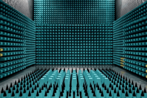
Anechoic Chamber with Ferrite and Hybrid Absorber
One final solution is to make your measurements within a shielded enclosure or chamber.
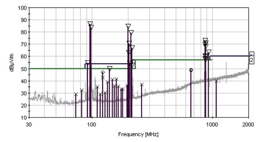
Open Area Test Site With Ambients (Shown By Triangles)
The main benefit to this is that ambient noise sources are significantly attenuated, normally by 80-110dB.
If you’re making radiated measurements, it’s important to use an anechoic chamber rather than a shielded room. Without absorbing material on the walls such as ferrite or hybrid absorber, waves will be free to reflect off the walls and ceiling making measurements unreliable and unrepeatable.
Conclusion
This article outlined several ways to expose signals that would otherwise not be measurable in your office environment.
Did I miss any tips? Let me know below…
Comments 1
Excellent and useful article. Correlating in-house to chamber measurements is a key component of every EMC job, and analyzer noise floor can be a confusing issue.